|
| |

Bernoulli
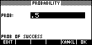
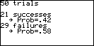
| This program is designed for use when students are
investigating the concept of Bernoulli Trials in probability. The user
nominates how many trials to perform, what the probability of success is
and the program reports how many successes were found. The results can be
stored into L0 if desired. |
 |
 |
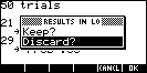
| If a graphical representation is needed then the
user can go to the HOME view and STO L0 into one of the Statistics aplet
columns. The default choice is to discard the results, which will empty
L0. |
 |
 |
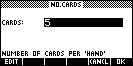
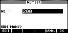
Hands of Cards
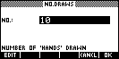
| For experimental probability problems involving
cards, this program will create and record any number of 'hands' of cards
of any specified size. For example, if 10 poker hands were needed
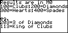
then the results are shown right. |
 |
 |
The results are stored in M0 and, because matrices
can't handle text, it is not possible to display "King of
Hearts" in the results. A code is used instead, where the hundreds
digit indicates the suit (100=Clubs, 200=Diamonds, 300=Hearts &
400=Spades) and the tens & units digits indicate the card value.
For example, an entry of 304 would be a 4 of Hearts,
while 212 would be a Queen of Diamonds.
Note: The results are stored in matrix
M0, which is not deleted at the end of the program. To save memory it is
worth deleting it when it is no longer needed. |
 |
 |
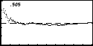
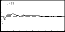
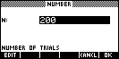
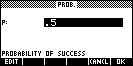
Long Run Prob
| Students generally accept as being reasonable that
the more experiments you perform, the more closely the experimental
probability approaches the theoretical probability. This program is
designed to show this visually. The user nominates a probability and
a number of trials and the program then displays the values of the
experimental probability as it changes with the number of trials. Visually
it becomes quite clear that the values are converging and also, more
importantly, that the values are wildly different for small numbers of
trials. |
 |
 |
| The dotted line on the graph shows the theoretical
probability value and the experimental probability is displayed at the top
of the screen as it changes. |
 |
 |
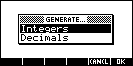
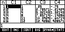
Random Numbers
| This program generates set of random numbers,
either integers or decimals. The results are stored into either a
list (L1...L5) or a column of the Statistics aplet (C1...C5). |
 |
 |
 |
|
 |
 |
 |
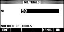
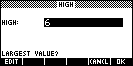
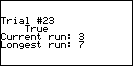
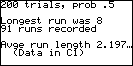
Avg Run Length
| The concept of average run length is
often useful in attempting to detect forgery of results. For example, if a
student were given the task of tossing a coin 200 times for homework and
decided to fake the results, they will often produce a fake which is 'too
random'. Although people understand intellectually that it is
possible to have runs of heads or tails, they usually don't take this into
account in their forgery. Investigating the average run length will often
show a value which is lower than the expected value of 0.5/[p(1-p)].
For example, suppose the student submitted 30
tosses of:
T H T H H T H T H H T H H T H T H T T T H T H T T H H T H T
The probability of an H according to this run is 0.5
exactly as expected, but what of the run length?
Breaking this into 'runs' gives:
T,H,T,HH,T,H,T,HH,T,HH,T,H,T,H,TTT,H,T,H,T,T,HH,T,H,T
This gives runs of:
1,1,1,2,1,1,1,2,1,2,1,1,1,1,3,1,1,1,1,1,2,1,1,1 giving an average run
length of 30/24 or 1.25.
The expected value is 0.5/[0.5*(1-0.5)] or 2. From
this one might suspect that the sample was faked, although the sample size
is clearly too small to be sure. |
| An interesting class investigation can be performed
by having each student perform an experiment like tossing a coin 200 times
and privately giving instructions to some students to fake their results, without
mentioning the concept of run length. Once all the results are
in, the class can be told that some students faked their results (but not
who or how many) and seeing if they can use run length to identify who
they were. |
 |
This program allows the student to investigate
average run length by having the computer 'toss the coins' (for any given
probability of sucess & number of trials) and give the average run
length it finds. The program reports its ongoing results as the
trials progress as well as the final totals. Change to the NUM view
to see the actual run lengths recorded.
If this experiment is recorded repeatedly and the
results are stored in columns C2 and C3 (C1 is used by the program) as
ordered pairs of (prob, av.run length) then they can be graphed as
bivariate data with a view to investigating and finding the rule of
0.5/[p(1-p)].
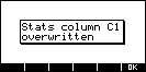
Note: Column C1 of the Statistics aplet
is overwritten by this program and some settings of the aplet may be
changed. |
 |
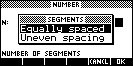
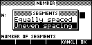
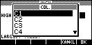
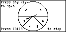
Spinner
| This program simulates a 'spinner' and
allows the student to collect experimental results. |
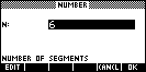 |
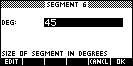
| The spinner can have any number of segments and
these segments can be either equally spaced or their sizes can be
specified in degrees. |
|
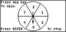 |
| To spin, press any key. When you press ENTER
the program will terminate. |
|
 |
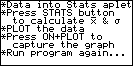
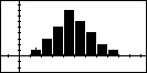
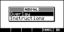
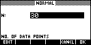
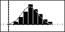
Overlay Normal
| It is often very helpful to be able to overlay a
normal curve with the same mean and standard deviation over the top of an
existing histogram. |
 |
 |
As the instructions say, there are
certain things that MUST be done before running the program.
 | The data must be graphed in the PLOT view. |
| The image must be captured for use by pressing
ON+PLOT |
This means hold down the ON button and, while still
holding it down, press PLOT.
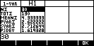
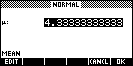
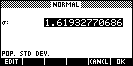
| In the NUM view, press STATS so that the values
of the mean and standard deviation can be calculated. If this is done
then the program will automatically import them when it is run. |
|
 |
| The image of the PLOT view is then
redisplayed and the equivalent normal curve is superimposed and displayed
until any key is pressed. |
 |
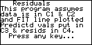
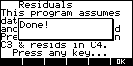
Residuals
| This is something that is easily done in the HOME
view but if you're lazy, this will do it for you. |
 |
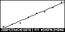 |
| The program will only run successfully if the data
has been graphed in the PLOT view first and the FIT line graphed (press
MENU & FIT). |
 |
 |
|